Understanding Manning's equation: the enduring workhorse of open-channel flows

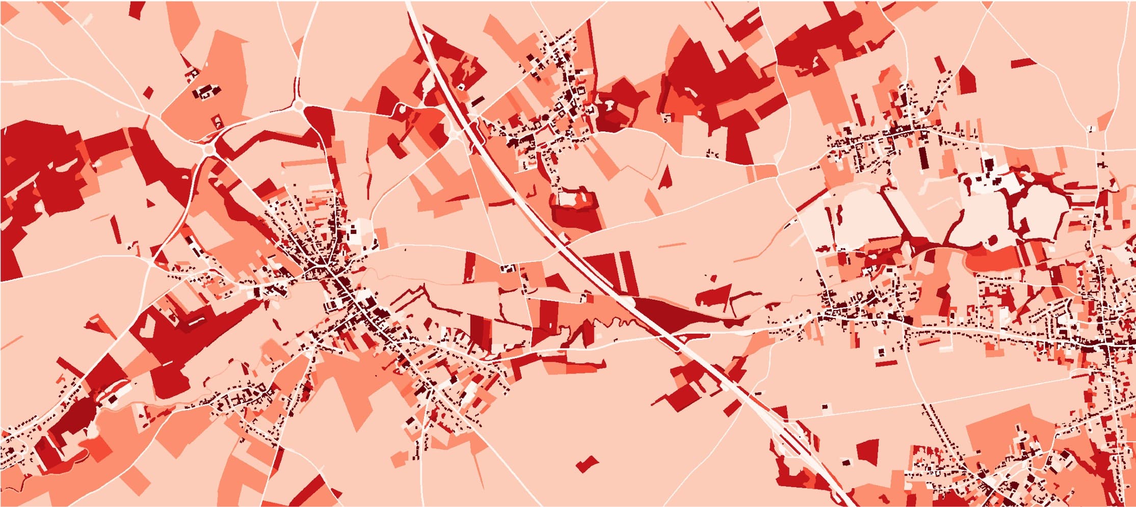
134 years old and still relevant: the life of Manning's equation

Robert Manning was not, by training, a hydraulic engineer. He was born in Normandy in 1816, the son of a soldier who had fought at Waterloo the year before, and moved to Waterford, Ireland, as a boy. He trained as an accountant. It was only in 1846, at the height of the Great Famine, that he was recruited into the Arterial Drainage Division of Ireland's Office of Public Works — an organisation that, in the following decades, would have him surveying and draining thousands of miles of rivers and channels across the country. Somewhere in that work he picked up a copy of d'Aubuisson des Voissons' Traité d'Hydraulique and developed what became a lifelong preoccupation with the mechanics of flowing water. By 1874 he was the Office's chief engineer.

By the late 1880s, open-channel hydraulics had a proliferation problem rather than a shortage: at least seven distinct formulas were in active use for predicting flow velocity in rivers and canals, proposed by Du Buat, Eytelwein, Weisbach, Saint-Venant, Neville, Darcy and Bazin, and Ganguillet and Kutter, each with its own coefficients and none obviously superior to the others. Manning, being rather pragmatic, didn't try to derive a better formula from first principles. He simply computed what each of the seven formulas predicted for a wide range of hydraulic radii — from 0.25 to 30 metres — averaged the results, and looked for a simple expression that reproduced that average curve. From that exercise, it turned out that a formula with the hydraulic radius (explained below) raised to the two-thirds power fit the averaged data better than anything with a square-root or first-power dependence. He presented the result to the Institution of Civil Engineers in Ireland on 4 December 1889, at the age of 73; the paper, "On the Flow of Water in Open Channels and Pipes," appeared in print in 1891.

There's a good, slightly ironic postscript to this story. Manning's formula involved a cube root, which was genuinely painful to compute by hand in the 1890s, so he later proposed an alternative without one — an equation that, among other things, awkwardly included barometric pressure as a variable, and which nobody adopted. Meanwhile, other engineers, working from his 1889 paper, had already noticed that the reciprocal of his coefficient corresponded closely to the roughness values that Ganguillet and Kutter had tabulated a decade earlier, and began quietly substituting those tabulated values in for practical use. The formula that carries Manning's name today — dimensionally awkward, missing a velocity-head correction term that wasn't even recognised as necessary until 1877 — is really a hybrid that later engineers assembled from his work and Kutter's, and it did not become the standard tool of the profession until Horace King's 1918 Handbook of Hydraulics put it in front of a generation of practising engineers.

None of that origin story would matter much if the formula hadn't kept working. It has now outlived seven or eight generations of alternative resistance formulas, survived the transition from slide rules to finite-volume solvers running on big computing clusters, and remains — unchanged in form — the roughness closure inside essentially every hydraulic model in use today, from a back-of-envelope check to a two-dimensional shallow-water solver simulating an entire flood plain. This longevity merits an explanation.

The equation

Manning's equation, in the form everyone uses, states that the average velocity of water moving through an open channel is:

$$V = \frac{1}{n} · R^{2/3} · S^{1/2}$$

and, since discharge is simply velocity times cross-sectional area,

$$Q = \frac{A}{n} · R^{2/3} · S^{1/2}$$

Every term here is doing specific physical work, and it's worth taking them one at a time.

$A$, the cross-sectional area of the flow, is the least mysterious term — it's just the area of water perpendicular to the direction of flow.

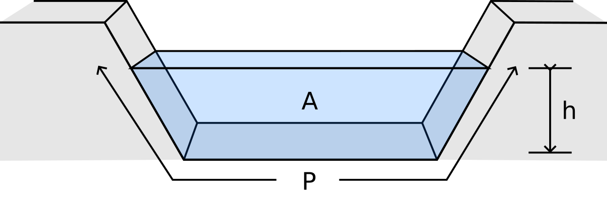
$R$, the hydraulic radius, is less obvious and more interesting. It's defined as $A$ divided by the wetted perimeter $P$ — the length of the boundary that is actually in contact with the water, excluding the free surface. The term is simply but incredibly elegant. The ratio combines the total area available to the flow to move through with the length of the channel’s solid boundary that is trying to resist it. So, $R$ can be thought of as a quantification of the relative ease with which water is able to flow though a channel cross-section.

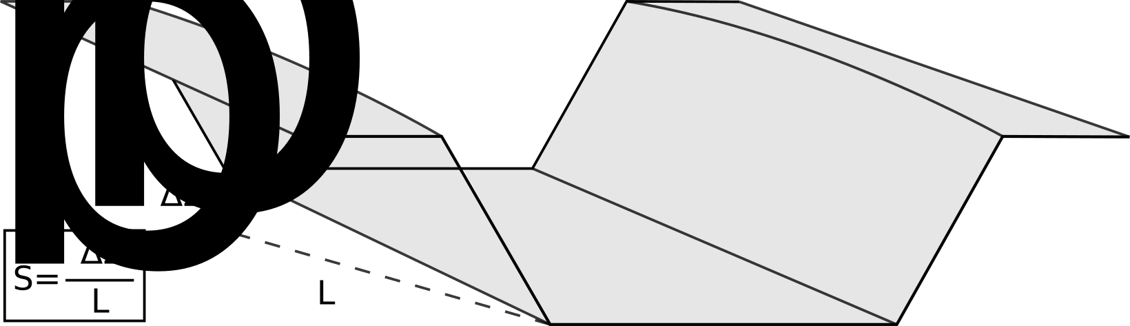
$S$, the slope, is the slope of the energy grade line — the rate at which the water is losing mechanical energy to friction per unit distance travelled. In the steady, uniform flow that Manning's equation strictly describes, the bed slope, the water-surface slope, and the energy slope all coincide, so in practice $S$ is usually just measured as the channel's longitudinal bed slope.

$n$, Manning's roughness coefficient, is where all the physics that the other three terms don't capture gets swept to. It stands in for the type and size of sediments on the bed, the shape and spacing of bedforms, vegetation, channel irregularity, sinuosity, obstructions — everything about the boundary, beyond its wetted perimeter, that generates resistance. This lumping is both the formula's great practical strength and, as the next section covers, its central weakness.

The $n$ problem

This is the part of Manning's equation that working hydraulic engineers have spend a lot of time arguing about, and for good reason: $n$ is not a material property in the way that, say, density or viscosity is. It cannot be measured directly on a sample of riverbed the way you'd measure the density of a rock. It is a fitted, situation-dependent number that, as stated before, has to absorb every source of resistance the other three terms of the equation don't already account for.

In practice, engineers reach for $n$ in one of two ways. The first is a lookup table — Chow's classic tabulation, still reproduced in essentially every hydraulics textbook, gives ranges for concrete-lined channels ($n$ ≈ 0.011–0.015), gravel beds ($n$ ≈ 0.025–0.040), and floodplains with dense brush ($n$ ≈ 0.070–0.160 or higher), among many other categories. The second, more rigorous approach is Cowan's method (Cowan, 1956), which builds $n$ up from components: a base value for the bed material, plus additive corrections for the degree of surface irregularity, the variability of the channel's cross-sectional shape along the reach, the frequency and size of obstructions, the density of vegetation, and the degree of meandering — then multiplies the whole sum by a correction factor for sinuosity. It's a more defensible process than picking a single number off a photograph, but it is still, at its core, expert judgement translated into arithmetic.

The consequences of getting that judgement wrong are worth quantifying, because they are easy to underestimate. If you are using Manning's equation forward — computing discharge from a known geometry, slope, and roughness — the relationship is direct: $Q$ is inversely proportional to $n$, so a 20% error (over- or under-estimation) in $n$ produces roughly 17% under-estimation or 25% over-estimation error, respectively, in the discharge. That is already a large error to be carrying on the back of a single, unmeasurable coefficient chosen by eye from a table of reference photographs.

The more consequential case, though, is the inverse problem that flood mapping actually depends on: given an expected discharge, what water level does it produce? For a wide channel, where the hydraulic radius is approximately equal to depth, Manning's equation reduces to $Q \propto h^{5/3}$, which rearranges to give depth as $h \propto n^{3/5}$. Differentiate that relationship and a 20% error in $n$ propagates into roughly a 12% error in predicted flood stage. On a floodplain, 12% of a meter or two of depth could be very significant — it is very often the difference between a hazard map that shows a house as dry or inundated. And this is before accounting for the fact that $n$ itself is not even constant for a given reach: it changes with stage, as vegetation that stands proud of the water at low flow submerges and flattens at high flow, as bed material mobilises and bedforms reorganise, and as the season changes what's growing on the banks. A single fixed $n$, applied across an entire flood hydrograph, is always at best a time-averaged approximation of a coefficient that is, in reality, drifting throughout the event it's being used to predict.

Limitations

Manning's equation applies, strictly, for steady, uniform flow — constant discharge, constant depth, constant velocity along the reach. Almost nobody uses it under those exact conditions. It's applied routinely to gradually varied flow (a backwater curve behind a bridge or weir) and to genuinely unsteady flow (a flood wave moving down a channel), on the working assumption that at each instant, at each cross-section, the flow behaves as if it were locally uniform — the same assumption that lets kinematic and diffusive-wave flood-routing models get away with using Manning's equation as their resistance law even though the flow they're simulating is, by definition, not steady.

The formula also degrades in specific, well-documented ways outside typical river conditions. In very shallow flow, where depth becomes comparable to the size of the roughness elements on the bed — a thin sheet of water flowing over cobbles, for instance — the assumption of a well-defined, depth-independent roughness breaks down, and $n$ effectively has to increase sharply as depth decreases to keep the equation honest. In vegetated channels the drag from stems and leaves is a strongly nonlinear function of how submerged the vegetation is, something a single roughness coefficient captures only crudely. And in steep, boulder-bed mountain streams — slopes above about 0.002, where large clasts can occupy a substantial fraction of the flow depth itself — Manning's equation with conventional $n$ values systematically underpredicts resistance, which is why alternatives like Jarrett's equation, which makes $n$ itself a function of slope and hydraulic radius rather than treating it as fixed, were developed specifically for that terrain.

Finally, there's a purely bureaucratic hazard worth flagging: the coefficient in front of the equation, $1/n$, is not universal. In SI units the coefficient is 1; in US customary units, because of the way the formula was anglicised in the early twentieth century, it's 1.486 (or 1.49, depending on the source). Dropping or duplicating that conversion factor is a well-known source of order-of-magnitude errors in software that mixes unit systems.

Contemporary use

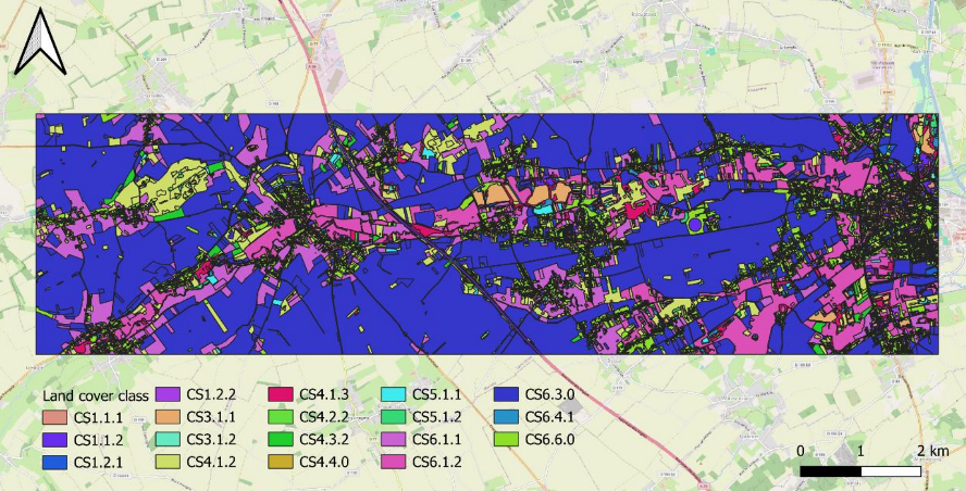
Despite everything in the previous two sections, Manning's equation continues to live. Why? Well, it is simple, it is calibratable against real gauge data with a single free parameter, and the engineering profession has accumulated well over a century of tabulated $n$ values, case studies, and institutional familiarity that would be enormously costly to discard. In solvers that use Manning’s equation as the roughness closure, the $n$ values are usually assigned based on land-cover data and/or bed-material zone from a calibration exercise that adjusts $n$, until modelled water levels match observed ones at gauging stations. In that sense the "problem" of $n$ is not really solved by these tools so much as delegated to calibration — the model doesn't need $n$ to be physically correct, only self-consistent enough to reproduce known events.

Now, before we close, and since we shall often focus on flood hazard and protection on this website — one quick application of Manning's equation is estimating bankful discharge — the flow that just fills a channel to the top of its banks before spilling onto the floodplain. The method is straightforward: survey or guess a representative channel cross-section, measure the reach-averaged bed or water-surface slope, and assign a roughness coefficient by comparing the reach to references — then solve Manning's equation directly for discharge.

And voila! With only a tape measure, a level, and a table of roughness photographs, an engineer could potentially get a feel for a channel's capacity. A fitting use for a formula built the same way: not derived from first principles in a laboratory, but assembled by someone who spent years walking riverbanks, comparing what worked, and writing down the average of everyone else's best guesses. A hundred and thirty-four years later, that remains, for most practical purposes, still a guess-good-enough before more sophisticated models step in.